17_OPTIMIZER-TRACE

Create:2025/05/31 b9f0d6b Update:2025-05-31

一镜到底 #

对于 MySQL 5.6 以及之前的版本来说，查询优化器就像是一个黑盒子一样，你只能通过 EXPLAIN 语句查看到最后优化器决定使用的执行计划，却无法知道它为什么做这个决策。这对于一部分喜欢刨根问底的小伙伴来说简直是灾难：“我就觉得使用其他的执行方案比 EXPLAIN 输出的这种方案强，凭什么优化器做的决定和我想的不一样呢？”

在 MySQL 5.6 以及之后的版本中，设计 MySQL 的大叔贴心的为这部分小伙伴提出了一个 optimizer trace 的功能，这个功能可以让我们方便的查看优化器生成执行计划的整个过程，这个功能的开启与关闭由 系统变量 optimizer_trace 决定，我们看一下：SHOW VARIABLES LIKE 'optimizer_trace';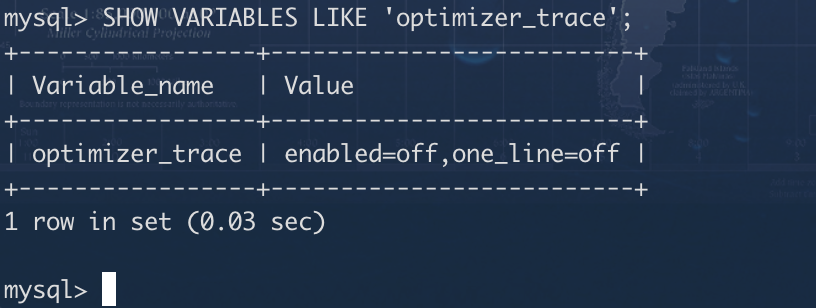

可以看到 enabled 值为 off ，表明这个功能默认是关闭的。

小贴士

one_line 的值是控制输出格式的，如果为 on 那么所有输出都将在一行中展示，不适合人阅读，所以我们就保持其默认值为 off 吧。

如果想打开这个功能，必须首先把 enabled 的值改为 on ，就像这样：
SET optimizer_trace="enabled=on";

然后我们就可以输入我们想要查看优化过程的查询语句，当该查询语句执行完成后，就可以到 information_schema 数据库下的 OPTIMIZER_TRACE 表 中查看完整的优化过程。这个 OPTIMIZER_TRACE 表有4个列，分别是：

QUERY ：表示我们的查询语句。
TRACE ：表示优化过程的JSON格式文本。
MISSING_BYTES_BEYOND_MAX_MEM_SIZE ：由于优化过程可能会输出很多，如果超过某个限制时，多余的文本将不会被显示，这个字段展示了被忽略的文本字节数
INSUFFICIENT_PRIVILEGES ：表示是否没有权限查看优化过程，默认值是0，只有某些特殊情况下才会是 1 ，我们暂时不关心这个字段的值。

完整的使用 optimizer trace 功能的步骤总结如下：

# 1. 打开optimizer trace功能 (默认情况下它是关闭的):
SET optimizer_trace="enabled=on";

# 2. 这里输入你自己的查询语句
SELECT ...;

# 3. 从OPTIMIZER_TRACE表中查看上一个查询的优化过程
SELECT * FROM information_schema.OPTIMIZER_TRACE;

# 4. 可能你还要观察其他语句执行的优化过程，重复上边的第2、3步
...

# 5. 当你停止查看语句的优化过程时，把optimizer trace功能关闭
SET optimizer_trace="enabled=off";

现在我们有一个搜索条件比较多的查询语句，它的执行计划如下：

EXPLAIN SELECT * FROM s1 WHERE
    key1 > 'z' AND
    key2 < 1000000 AND
    key3 IN ('a', 'b', 'c') AND
    common_field = 'abc';
# placeholder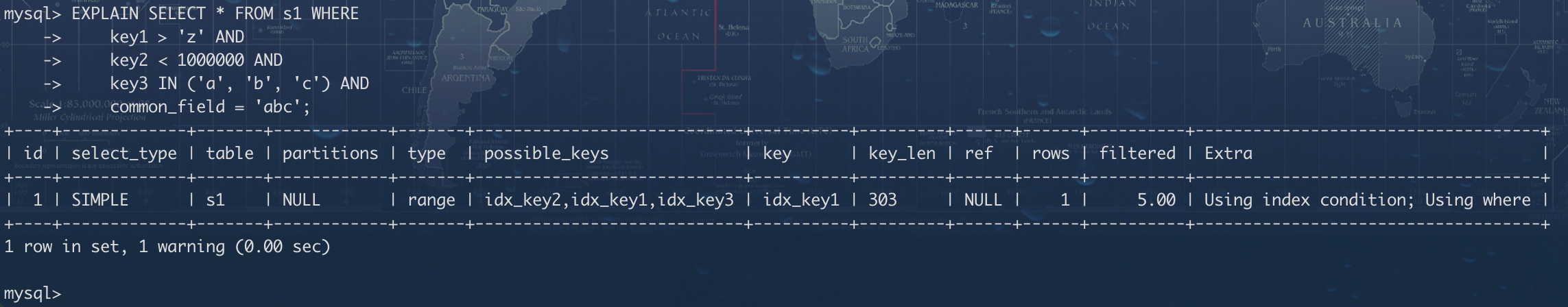

可以看到该查询可能使用到的索引有3个，那么为什么优化器最终选择了 idx_key2 而不选择其他的索引或者直接全表扫描呢？这时候就可以通过 otpimzer trace 功能来查看优化器的具体工作过程：

SET optimizer_trace="enabled=on";

SELECT * FROM s1 WHERE
    key1 > 'z' AND
    key2 < 1000000 AND
    key3 IN ('a', 'b', 'c') AND
    common_field = 'abc';

SELECT * FROM information_schema.OPTIMIZER_TRACE\G

我们直接看一下通过查询 OPTIMIZER_TRACE 表得到的输出（我使用 # 后跟随注释的形式为大家解释了优化过程中的一些比较重要的点，大家重点关注一下）：

mysql> SELECT * FROM information_schema.OPTIMIZER_TRACE\G
*************************** 1. row ***************************
                            QUERY: SELECT * FROM s1 WHERE
    key1 > 'z' AND
    key2 < 1000000 AND
    key3 IN ('a', 'b', 'c') AND
    common_field = 'abc'                                                # 分析的查询语句是什么
TRACE: {                                                                # 优化的具体过程
    "steps": [
        {
        "join_preparation": {                                           # prepare阶段
            "select#": 1,
            "steps": [
            {
                "IN_uses_bisection": true
            },
            {
                "expanded_query": "/* select#1 */ select `s1`.`id` AS `id`,`s1`.`key1` AS `key1`,`s1`.`key2` AS `key2`,`s1`.`key3` AS `key3`,`s1`.`key_part1` AS `key_part1`,`s1`.`key_part2` AS `key_part2`,`s1`.`key_part3` AS `key_part3`,`s1`.`common_field` AS `common_field` from `s1` where ((`s1`.`key1` > 'z') and (`s1`.`key2` < 1000000) and (`s1`.`key3` in ('a','b','c')) and (`s1`.`common_field` = 'abc'))"
            }
            ]
        }
        },
        {
        "join_optimization": {                                          # optimize阶段
            "select#": 1,
            "steps": [
            {
                "condition_processing": {                               # 处理搜索条件
                "condition": "WHERE",                                   # 原始搜索条件
                "original_condition": "((`s1`.`key1` > 'z') and (`s1`.`key2` < 1000000) and (`s1`.`key3` in ('a','b','c')) and (`s1`.`common_field` = 'abc'))",
                "steps": [
                    {
                    "transformation": "equality_propagation",           # 等值传递转换
                    "resulting_condition": "((`s1`.`key1` > 'z') and (`s1`.`key2` < 1000000) and (`s1`.`key3` in ('a','b','c')) and (`s1`.`common_field` = 'abc'))"
                    },
                    {
                    "transformation": "constant_propagation",           # 常量传递转换
                    "resulting_condition": "((`s1`.`key1` > 'z') and (`s1`.`key2` < 1000000) and (`s1`.`key3` in ('a','b','c')) and (`s1`.`common_field` = 'abc'))"
                    },
                    {
                    "transformation": "trivial_condition_removal",      # 去除没用的条件
                    "resulting_condition": "((`s1`.`key1` > 'z') and (`s1`.`key2` < 1000000) and (`s1`.`key3` in ('a','b','c')) and (`s1`.`common_field` = 'abc'))"
                    }
                ]
                }
            },
            {
                "substitute_generated_columns": {                       # 替换虚拟生成列
                }
            },
            {
                "table_dependencies": [                                 # 表的依赖信息
                {
                    "table": "`s1`",
                    "row_may_be_null": false,
                    "map_bit": 0,
                    "depends_on_map_bits": [
                    ]
                }
                ]
            },
            {
                "ref_optimizer_key_uses": [
                ]
            },
            {
                "rows_estimation": [                                    # 预估不同单表访问方法的访问成本
                {
                    "table": "`s1`",
                    "range_analysis": {
                    "table_scan": {                                     # 全表扫描的行数以及成本
                        "rows": 10039,
                        "cost": 2106.9
                    },
                    "potential_range_indexes": [                        # 分析可能使用的索引
                        {
                        "index": "PRIMARY",                             # 主键不可用
                        "usable": false,
                        "cause": "not_applicable"
                        },
                        {
                        "index": "idx_key2",                            # idx_key2 可能被使用
                        "usable": true,
                        "key_parts": [
                            "key2"
                        ]
                        },
                        {
                        "index": "idx_key1",                            # idx_key1 可能被使用
                        "usable": true,
                        "key_parts": [
                            "key1",
                            "id"
                        ]
                        },
                        {
                        "index": "idx_key3",                            # idx_key3 可能被使用
                        "usable": true,
                        "key_parts": [
                            "key3",
                            "id"
                        ]
                        },
                        {
                        "index": "idx_key_part",                        # idx_keypart 不可用
                        "usable": false,
                        "cause": "not_applicable"
                        }
                    ],
                    "setup_range_conditions": [
                    ],
                    "group_index_range": {
                        "chosen": false,
                        "cause": "not_group_by_or_distinct"
                    },
                    "analyzing_range_alternatives": {                   # 分析各种可能使用的索引的成本
                        "range_scan_alternatives": [
                        {
                            "index": "idx_key2",                        # 使用 idx_key2 的成本分析
                            "ranges": [                                 # 使用 idx_key2 的范围区间
                            "NULL < key2 < 1000000"
                            ],
                            "index_dives_for_eq_ranges": true,          # 是否使用 index dive
                            "rowid_ordered": false,                     # 使用该索引获取的记录是否按照主键排序
                            "using_mrr": false,                         # 是否使用 mrr
                            "index_only": false,                        # 是否是索引覆盖访问
                            "rows": 10000,                              # 使用该索引获取的记录条数
                            "cost": 12001,                              # 使用该索引的成本
                            "chosen": false,                            # 是否选择该索引
                            "cause": "cost"                             # 因为成本太大所以不选择该索引
                        },
                        {
                            "index": "idx_key1",
                            "ranges": [
                            "z < key1"
                            ],
                            "index_dives_for_eq_ranges": true,
                            "rowid_ordered": false,
                            "using_mrr": false,
                            "index_only": false,
                            "rows": 1,
                            "cost": 2.21,
                            "chosen": true
                        },
                        {
                            "index": "idx_key3",
                            "ranges": [
                            "a <= key3 <= a",
                            "b <= key3 <= b",
                            "c <= key3 <= c"
                            ],
                            "index_dives_for_eq_ranges": true,
                            "rowid_ordered": false,
                            "using_mrr": false,
                            "index_only": false,
                            "rows": 3,
                            "cost": 6.61,
                            "chosen": false,
                            "cause": "cost"
                        }
                        ],
                        "analyzing_roworder_intersect": {               # 分析使用索引合并的成本
                        "usable": false,
                        "cause": "too_few_roworder_scans"
                        }
                    },
                    "chosen_range_access_summary": {                    # 对于上述单表查询 s1 最优的访问方法
                        "range_access_plan": {
                        "type": "range_scan",
                        "index": "idx_key1",
                        "rows": 1,
                        "ranges": [
                            "z < key1"
                        ]
                        },
                        "rows_for_plan": 1,
                        "cost_for_plan": 2.21,
                        "chosen": true
                    }
                    }
                }
                ]
            },
            {
                "considered_execution_plans": [                         # 分析各种可能的执行计划
                                                                        #（对多表查询这可能有很多种不同的方案，单表查询的方案上边已经分析过了，直接选取 idx_key1 就好）
                {
                    "plan_prefix": [
                    ],
                    "table": "`s1`",
                    "best_access_path": {
                    "considered_access_paths": [
                        {
                        "rows_to_scan": 1,
                        "access_type": "range",
                        "range_details": {
                            "used_index": "idx_key1"
                        },
                        "resulting_rows": 1,
                        "cost": 2.41,
                        "chosen": true
                        }
                    ]
                    },
                    "condition_filtering_pct": 100,
                    "rows_for_plan": 1,
                    "cost_for_plan": 2.41,
                    "chosen": true
                }
                ]
            },
            {
                "attaching_conditions_to_tables": {                     # 尝试给查询添加一些其他的查询条件
                "original_condition": "((`s1`.`key1` > 'z') and (`s1`.`key2` < 1000000) and (`s1`.`key3` in ('a','b','c')) and (`s1`.`common_field` = 'abc'))",
                "attached_conditions_computation": [
                ],
                "attached_conditions_summary": [
                    {
                    "table": "`s1`",
                    "attached": "((`s1`.`key1` > 'z') and (`s1`.`key2` < 1000000) and (`s1`.`key3` in ('a','b','c')) and (`s1`.`common_field` = 'abc'))"
                    }
                ]
                }
            },
            {
                "refine_plan": [                                        # 再稍稍的改进一下执行计划
                {
                    "table": "`s1`",
                    "pushed_index_condition": "(`s1`.`key1` > 'z')",
                    "table_condition_attached": "((`s1`.`key2` < 1000000) and (`s1`.`key3` in ('a','b','c')) and (`s1`.`common_field` = 'abc'))"
                }
                ]
            }
            ]
        }
        },
        {
        "join_execution": {                                             # execute 阶段
            "select#": 1,
            "steps": [
            ]
        }
        }
    ]
}
MISSING_BYTES_BEYOND_MAX_MEM_SIZE: 0                                    # 因优化过程文本太多而丢弃的文本字节大小，值为 0 时表示并没有丢弃
          INSUFFICIENT_PRIVILEGES: 0                                    # 权限字段
1 row in set (0.01 sec)

mysql>

大家看到这个输出的第一感觉就是这文本也太多了点儿吧，其实这只是优化器执行过程中的一小部分，设计 MySQL 的大叔可能会在之后的版本中添加更多的优化过程信息。不过杂乱之中其实还是蛮有规律的，优化过程大致分为了三个阶段：

prepare 阶段
optimize 阶段
execute 阶段

我们所说的基于成本的优化主要集中在 optimize 阶段，对于单表查询来说，我们主要关注 optimize 阶段的 “rows_estimation” 这个过程，这个过程深入分析了对单表查询的各种执行方案的成本；对于多表连接查询来说，我们更多需要关注 “considered_execution_plans” 这个过程，这个过程里会写明各种不同的连接方式所对应的成本。反正优化器最终会选择成本最低的那种方案来作为最终的执行计划，也就是我们使用 EXPLAIN 语句所展现出的那种方案。

如果有小伙伴对使用 EXPLAIN 语句展示出的对某个查询的执行计划很不理解，大家可以尝试使用 optimizer trace 功能来详细了解每一种执行方案对应的成本，相信这个功能能让大家更深入的了解 MySQL 查询优化器。